In this post, I will discuss a character model that I have been using to extract references to semantic entities (like payment amounts) in natural text. The intention here is to describe an elegant, small-scale machine learning model that can be applied as a simple alternative to complex, hard-coded logic. Analysis of this model also hints at many deeper, modern problems in sequential models, which we briefly explore.

Throughout this discussion, we will consider the problem of identifying references to payment amounts in text as a grounding example. This example is good because while we could likely design a decent heuristic algorithm for this task, such an algorithm would likely be highly complex and conditional because natural-language references to payment amounts can take many different forms. For instance, consider the fact that payment amounts may or may not include a currency symbol or abbreviation ($400, 400, 400€, or 400cad) and that some people may include comma (or sometimes period) separators (1650, $1,650, or £1.650,00) into their numbers. Furthermore, the problem is made more difficult because numerical characters often refer to things other than payment amounts such as dates, which themselves can be expressed in a variety of ways.

We’ve chosen to tackle this problem instead with a small machine learning model. An example of our model’s output is seen below:

The model that produces this was trained using less than 100 hand labeled examples in about a minute. It contains less than 500 parameters, consuming 3.7kB when serialized resulting in fast inference performance. The model achieves very usable accuracy in excess of 90% and is easy to ship and deploy in production environments.

The source code for this project can be found here along with the pre-built models I’ve trained for parsing payment amounts. It is worth noting that the data used to train these models follows a distribution that may not match the data for your use case exactly and so model performance for you may be lower than the numbers reported here. I will be releasing the training data for this project in the near future and intend also to continue writing about this work. Check back here later for more updates or feel free to reach out to me if you are interested in contributing yourself.

The remaining sections below are for those interested in a more detailed discussion of our work. We give a mathematical formulation of the model along with some of its expected mathematical properties before finally discussing our measurements for model and inference performance.

Mathematical Description

One can describe our model to be a linear, recurrent model with a simple auto-regressive state. Alternatively, for those who have studied time series methods, our model can be thought of as a \((0,1)\) normalized ARMA model in which the moving average noise pattern takes the form of non-independent bernoulli events instead of i.i.d. gaussians.

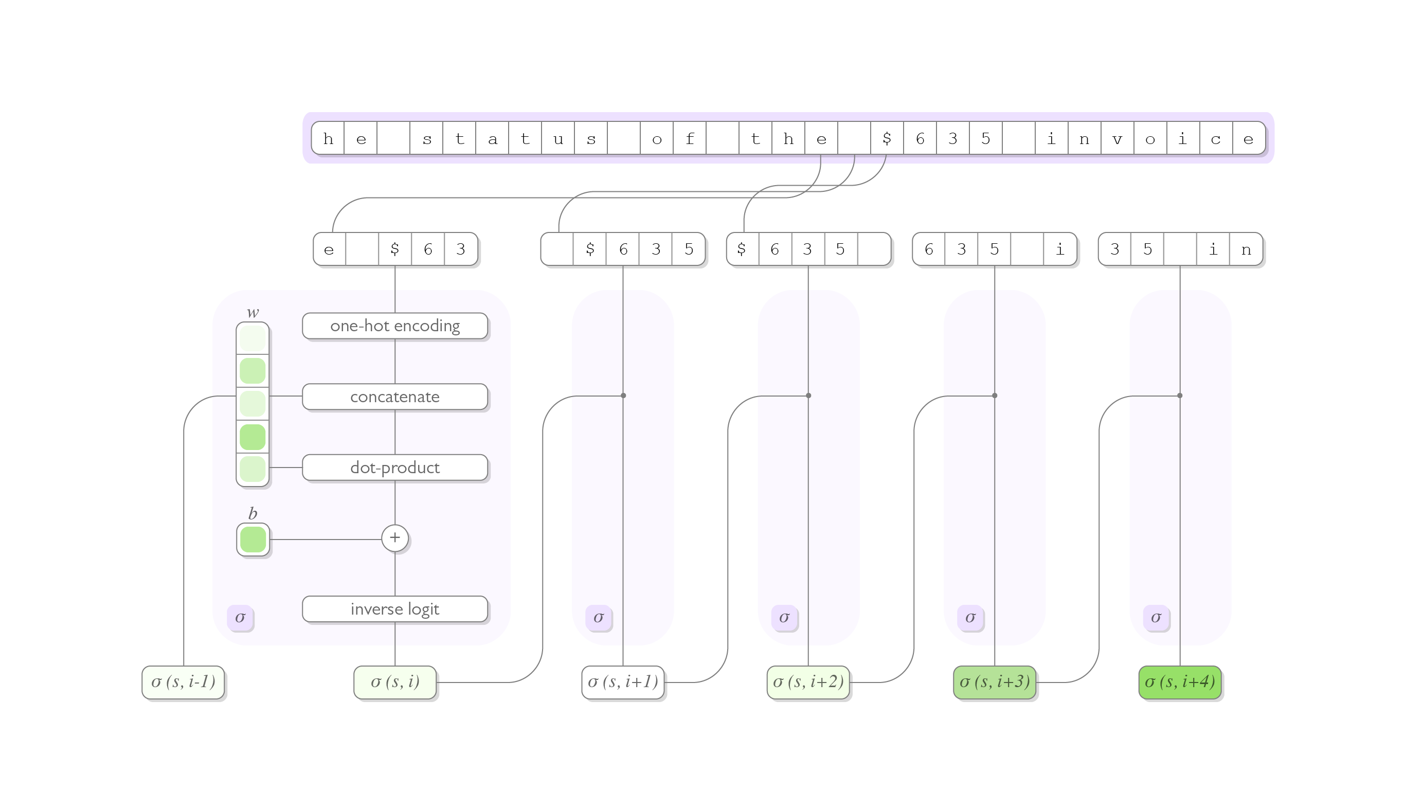
We start by taking a fixed, finite alphabet \(\mathcal{A}\) of characters of size \(N_\mathcal{A}\). A string of text takes the form of a sequence of characters \(s = c_1, c_2, \ldots\) drawn from \(\mathcal{A}\). We pose a binary classification model \(\sigma(s, i)\) which predicts whether to consider the character at some index \(i\) to be a part of a payment amount.

The mathematical expression for our model is given by:

\[\sigma(s, i) = \text{logit}^{-1}\left(\zeta \sigma(s, i - 1) + \sum_{j=0}^{W N_\mathcal{A}} \phi_j v(i)_j + b\right)\]

where \(\sigma(s, i - 1)\) is the output of our model on the previous character, \(v(i) \in \mathbb{R}^{W N_\mathcal{A}}\) is a vector encoding of the characters in a size \(W\) window about character \(i\),and \(\zeta\), \(b\), and \(\phi\) are learnable parameters. The inverse logit function is given by the formula seen below, and is applied to normalize the model’s output to the range \((0, 1)\).

\[\text{logit}^{-1}(x) = \frac{\exp(x)}{1 + \exp(x)}\]

The diagram below summarizes what we’ve described here:

It is worth noting that the model described here has considerable similarities to an ARMA(\(1\), \(WN_\mathcal{A}\)) time series model. This similarity suggests to us some interesting training strategies based on the Yule-Walker equations though we will save that discussion for another day.

Training Algorithm

Our model is naively trained using a sibling of the XENT training algorithm for RNNs where the cross-entropy loss is substituted with its binary logistic regression counterpart. In particular, we use SGD to minimize the following loss function:

\[\mathcal{L}(\sigma, \mathcal{D}) = -\sum_{s, l \in \mathcal{D}} \sum_{i=1}^{|s|} l_i \sigma(s, i)_{l_{i - 1}} + (1 - l_i) (1 - \sigma(s, i)_{l_{i - 1}})\]

where \(\mathcal{D}\) is a set of training data consisting of strings \(s\) and character-level labels \(l\), and where \(\sigma(s, i)_{l_{i - 1}}\) is our model’s output when its recurrent dependence on \(\sigma(s, i - 1)\) is replaced by the ground truth indicator \(l_{i - 1}\).

This method of training is equivalent to maximum likelihood estimation for a binary logistic classifier when each character-level classification is taken to be independent from the other (despite this obviously not being the case). We have found in practice that training in this way leads to working models but it is worth noting that that there are two significant reservations that one might have in its use.

First is the problem of exposure bias. One may have noticed that our model admits a conspicuous difference with its train-time and inference-time computation in that ground-truth priors are used during training in place of \(\sigma(s, i - 1)\) but not during inference. This divergence is known as exposure bias and it turns out to be a major pragmatic problem in recurrent sequence-generating models because small errors in output during inference can compound themselves later in the sequence. This has led general-purpose NLP models to move away from XENT to more robust training methods like REINFORCE.

Exposure bias is not as serious of a practical problem in our use case because the semantic rules represented by our model are considerably simpler than the general language models. However, it does present a interpretative problem as it unclear whether we are modeling each binary output character as dependent directly on the previous character (as described by the training paradigm) or if we are modeling it as dependent on a more abstract unobserved variable (as described by the inference paradigm). Firmly grounding this ambiguity has implications for the theoretical elegance of our model - expect an in-depth post on this topic in the near future.

Experiments

Initial experiments with our proposed autoregressive character model involved training a model to segment monetary reference from natural language text. Our initial experiment were done by training a model on a very small (\(N=80\)) dataset which is documented here. Hyper-parameters were chosen intuitively rather procedurally though we a use a window-shift of one so as to make use of proceeding currency symbols when identifying the beginning of segments.

We evaluated our model using a full leave-one-out cross validation on our dataset by training a fresh model to evaluate each full string, leaving the selected string out of the train set. It is worth noting here that we are treating each string as the “atomic” data point instead of the smaller subset of characters that we use to make a prediction at a single character.

Though a more in-depth look at more suitable measurement methods is probably warranted, we will give out initial report of model performance given in model accuracy. Since we are with working with whole strings as the atomic unit of data, the model response for a given string takes the form of a sequence of predictions (one for each character). We consider a string to be correctly labeled only if the model’s output sequence matches the ground truth exactly. This evaluation method may not be suitable for all data as perfect alignment of data for very long strings is probably unlikely. Fortunately, our dataset is such that each individual string is relatively short (typically less than 200 characters per string) so this method gives us a reasonable method of measuring model performance.

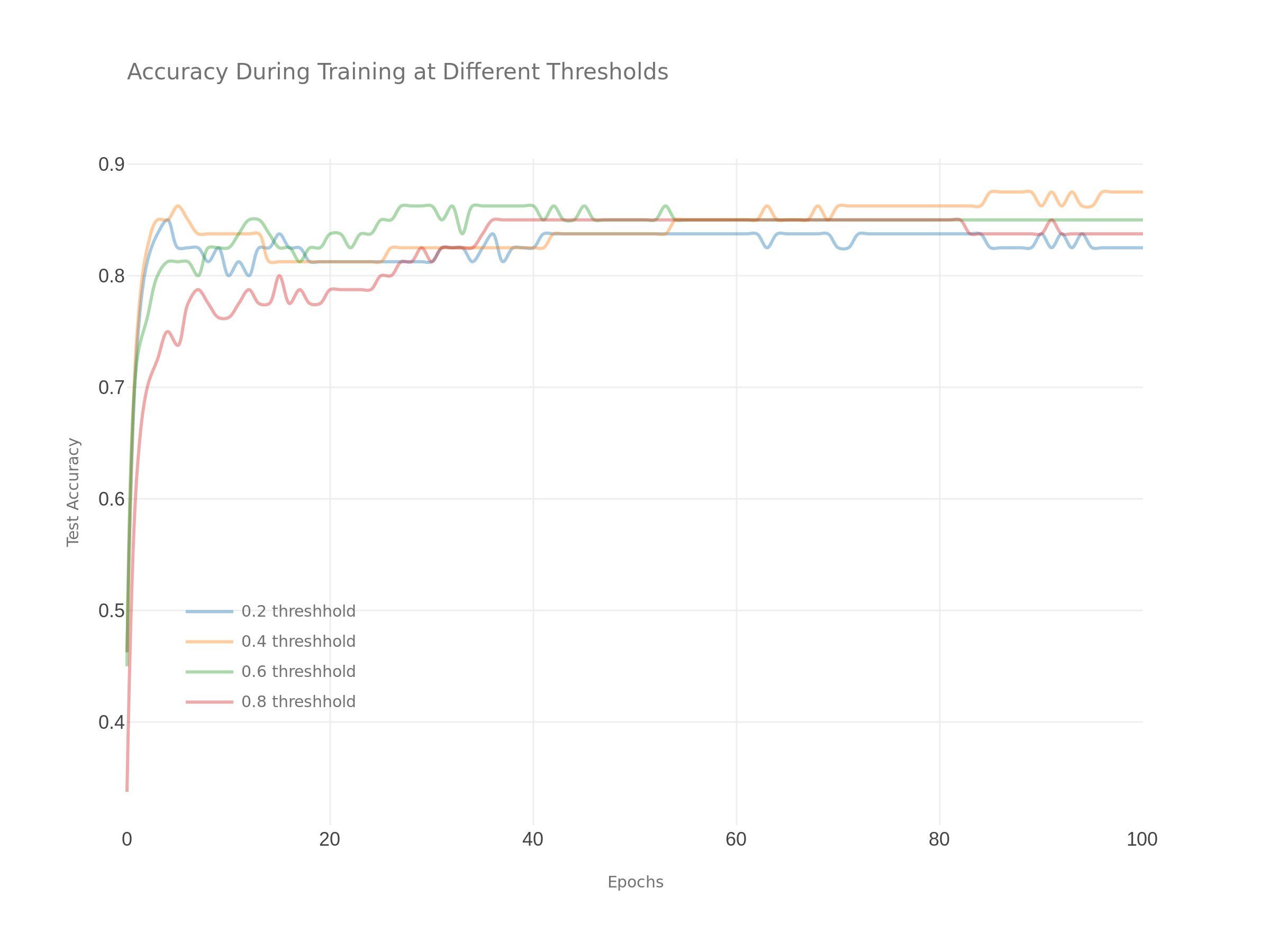
The follow plot shows how accuracy improves over the course of the training process for a few select threshold levels. Generally, we interpret this plot to show that our model has reached a reasonable state of convergence without any obvious signs of over fitting. In addition, this plot suggests a general-usage cutoff threshold of about 0.4.

---