I’ve written a few times on Euler Discretization. For functions \(h\) of one-dimension on a fixed compact domain, it’s known that Euler Discretization, taking \(N\) steps, exhibits maximum numerical error bounded by \(O(N^{-1})\) with time complexity that is bounded by \(O(N)\). Memory, if we choose to keep a record of all the intermediate values of \(h\), is also \(O(N)\).

This can be pretty simply demonstrated explicitly. Taking as an example, the simple linear ODE for a function \(h: \mathbb{R} \rightarrow \mathbb{R}\) given by:

\[h'(t) = w h(t) + b \qquad \qquad h(0) = h_0\]

for constants, \(w, b \in \mathbb{R}\) on the compact interval \([0, 1]\), this initial value problem has a known closed form solution:

\[h(t) = \exp(w t) \left(\frac{b}{w} + y_0\right) - \frac{b}{w}\]

Since the precise solution is known, we can compute the error of Euler Discretization as a function of the step size argument. Here is that relation plotted along with the associated memory and time costs.

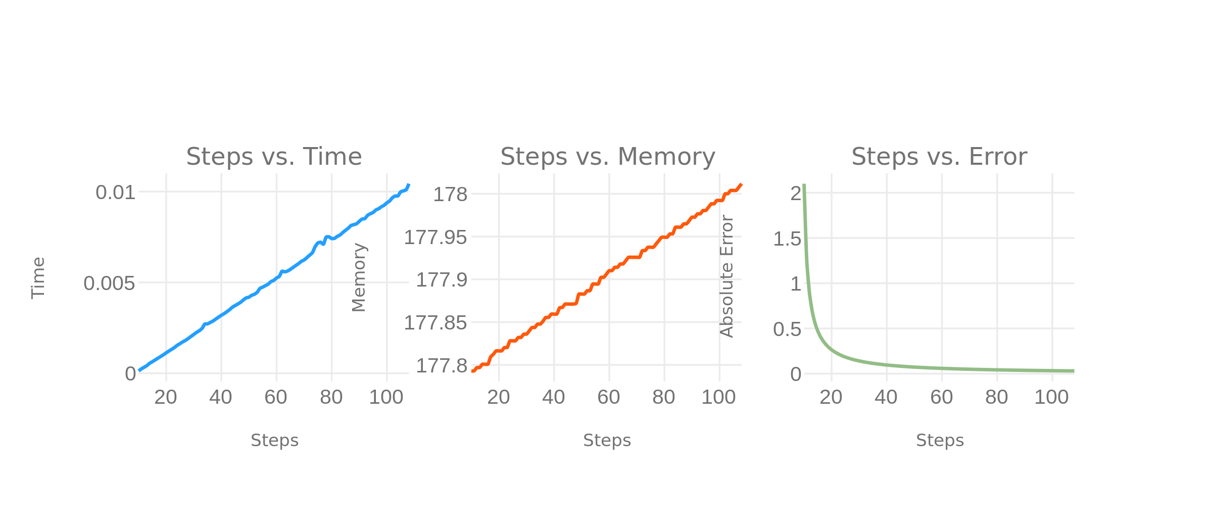
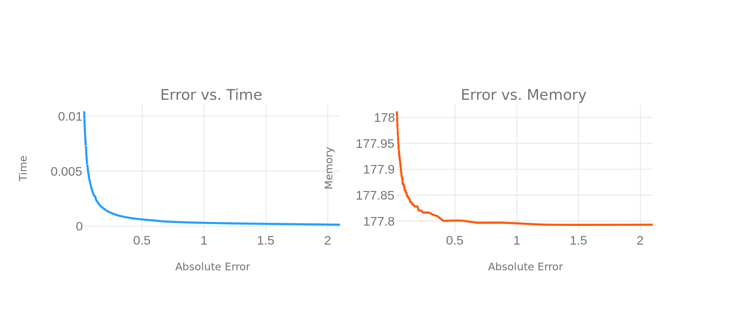
Since we typically express application requirements in terms of error and time/memory performance, we can convert the asymptotic bounds we give above (which are expressed as a function of steps) into a tradeoff between memory/time performance and solver precision. We start with the follow three relations:

\[\epsilon \sim O(N^{-1}) \quad m \sim O(N) \quad t \sim O(N)\]

And we derive that \(m, t \sim O(\epsilon^{-1})\). This is seen empirically as well:

The experiments on this page are run as a Jupyter notebook that can be found here.