Deep learning frameworks like Tensorflow and PyTorch have made it easy to abstract the the problem of automatic gradient computation for the vast majority of machine learning practitioners. The dominant pattern of differentiation in modern day deep learning, backpropagation, has become more or less synonymous with automatic differentiation in general despite there being problems that would benefit from other differentiation patterns. Today, we’ll discuss how the cost of auto-differentiation depends on the order we choose to algorithmically apply chain rule, focusing particularly on forward and reverse mode patterns. We’ll mostly avoid discussing other methods of derivative computation like symbolic and numerical differentiation which have limited applications in machine learning.

Suppose we have a sequence of functions \(f_k: \mathbb{R}^{n_k} \rightarrow \mathbb{R}^{n_{k+1}}\) which we compose cumulatively to obtain another sequence \(F_k:\mathbb{R}^{n_1} \rightarrow \mathbb{R}^{n_{k+1}}\) as follows:

the chain rule expresses that we can compute the derivative \(dF_k \vert_x\) as a series of matrix multiplications:

Since matrix multiplication is associative, we expect that the order we perform these matrix multiplications does not affect the end result. However, it’s often overlooked that that the number of FLOPs needed to obtain this result actually does vary depending on our choice of associativity.

Forward-mode differentiation computes \(DF_k\) as \(Df_k ( \ldots ( Df_2 ( Df_1) ) \ldots )\). This computation costs us (very roughly) \(n_1 \sum_{i=2}^k n_i n_{i+1}\) floating point operations whereas reverse-model differentiation, computing \(DF_k\) in the inverse order via \(( \ldots ( ( Df_k ) Df_{k-1} ) \ldots ) Df_1\), requires \(n_{k+1} \sum_{i=2}^k n_i n_{i-1}\) FLOPs.

Between these two options, the ideal choice depends on the relative sizes of \(n_1\) and \(n_{k+1}\). When \(n_{k+1} \ll n_1\), it’s clear that reverse-mode differentiation requires less computation. In machine learning applications gradients are typically computed on scalar-valued loss-function functions with high-dimensional inputs. As such, typically we have \(n_{k+1} = 1\) and a large value for \(n_1\), presenting a scenario where reverse-mode differentiation is a computationally more efficient choice.

Choosing to use backpropagation unfortunately has an additional memory cost over forward-mode differentiation. Note that computing \(Df_i\) requires us to know the activation \(F_{i-1}(x)\). In forward-mode differentiation, this can be done efficiently with constant memory because we need access to each \(F_{i-1}(x)\) activation for calculating derivatives in the same order that we compute them in the forward pass:

Inputs:
  composed functions : fs = [f1, ..., fk]
  derivatives        : dfs = [Df1, ..., Dfk]
  input point        : x

dFi = 1
aFi = x
for i in range(k):
    dFi = dfs[i](aFi) * dFi
    aFi = fs[i](aFi)
return dFi

However, in reverse-mode differentiation, we need to access intermediate activation in the inverse order that they must be computed so we must cache intermediate activations to avoid recomputing the forward pass for every single \(Df_i\):

Inputs:
  composed functions : fs = [f1, ..., fk]
  derivatives        : dfs = [Df1, ..., Df_k]
  input point        : x

aFis = [x]
for i in range(k):
  aFis.append(fs[i](aFis[-1])

dFi = 1
for i in range(k-1, -1, -1):
    dFi = dfs[i](aFis[i]) * dFi

return dFi

In summary, while forward-mode differentiation can be done in \(O(1)\) memory, reverse-mode differentiation requires memory roughly linear in the number of functions composed \(O(k)\).

Finally, it is also worth noting that we can choose to associate chain rule components in any arbitrary order. For a given sequence of intermediate dimensions \(n_1, \ldots n_{k+1}\), the time-optimal association is called the optimal Jacobian accumulation and will generally not be purely forward or reverse-mode. Finding the OJA for an arbitrary computational graph is NP-complete though perhaps, this can be done more efficiently for the linear, non-dependent computation graph described in our working example.

Experiments

We’ve run some experiments to validate the theoretical results presented here in the form of a comparison between the performance characteristics between forward-mode and reverse-mode auto-differentiation. These experiments use the following function to retrieve differentiation targets where we are interested in how time and memory consumption varies with function depth, and intermediate dimensionality of our function:

def get_fn_to_diff(n_start, n_end, n_middle, n_layers):
    def fn(x):
        x = np.tanh(np.matmul(np.zeros((n_middle, n_start)), x))
        for i in range(n_layers):
            x = np.tanh(np.matmul(np.zeros((n_middle, n_middle)), x))
        return np.tanh(np.matmul(np.zeros((n_end, n_middle)), x))

    return fn

The following measurements show that scaling of forward-mode differentiation compute complexity is sensitive to the size of the input dimension relative to the size of the middle dimensions and output dimensions while the scaling of reverse-mode differentiation compute complexity is sensitive to the size of the output dimension relative to the size of the middle dimensions and input dimensions:

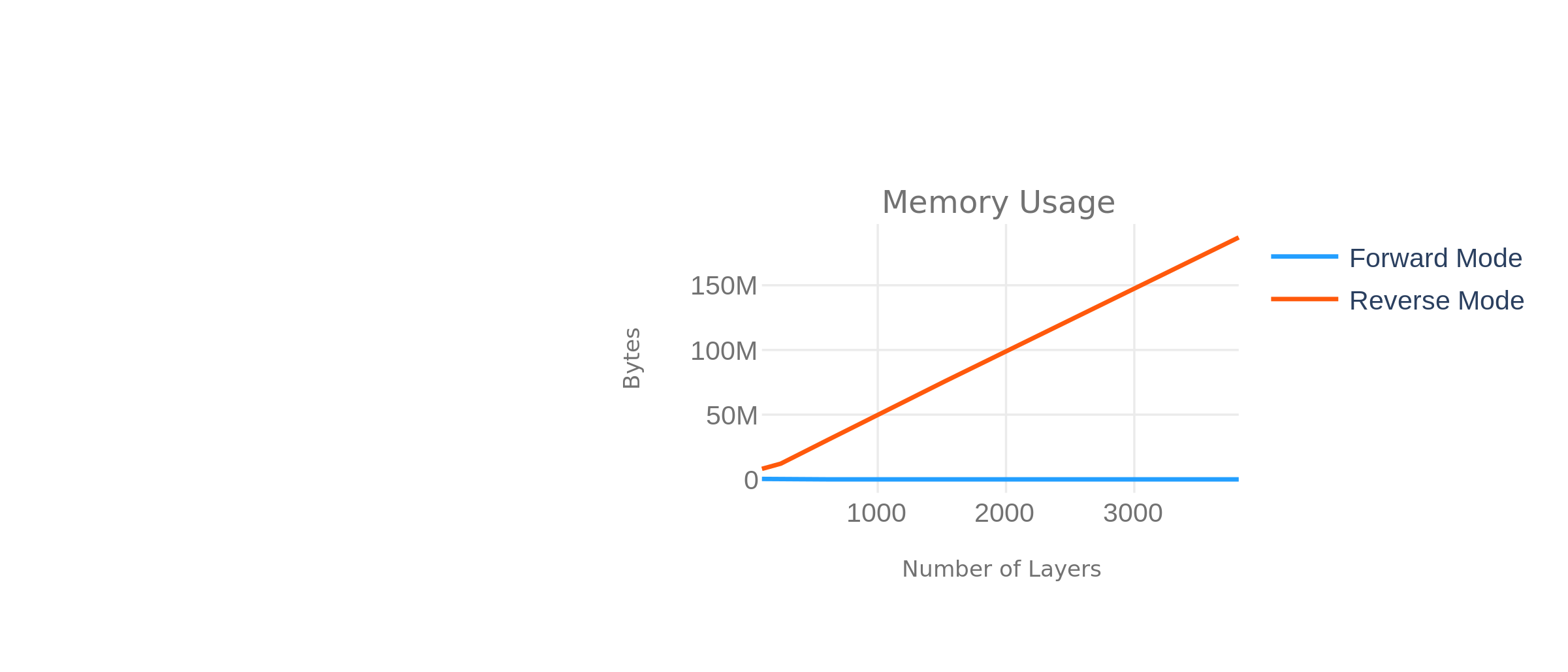
Similarly, our experiments show that differentiating deeper functions costs us linear memory only in reverse-mode auto-differentiation but not when using forward-mode auto-differentiation:

Code used to run our experiments can be found here.